
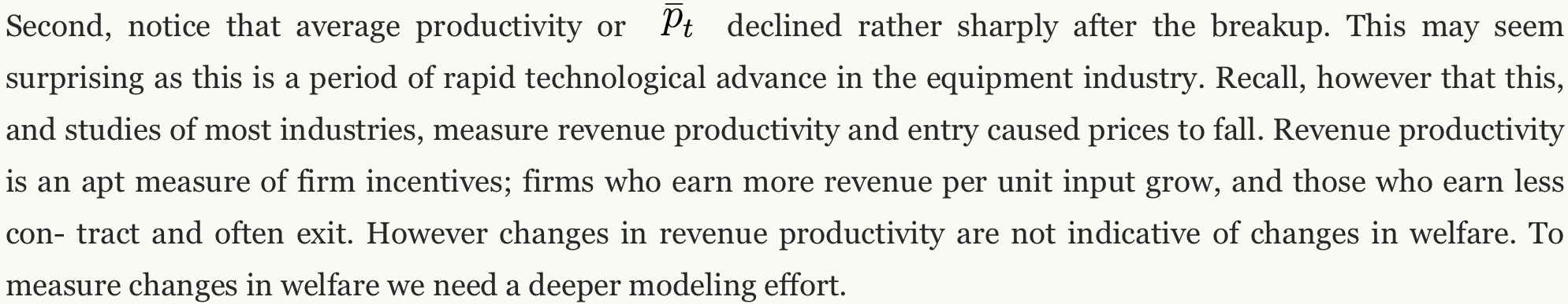
The Network Law Review is pleased to present you with a special issue curated by the Dynamic Competition Initiative (“DCI”). Co-sponsored by UC Berkeley and the EUI, the DCI seeks to develop and advance innovation-based dynamic competition theories, tools, and policy processes adapted to the nature and pace of innovation in the 21st century. This special issue brings together contributions from speakers and panelists who participated in DCI’s second annual conference in October 2024. This article is authored by Ariel Pakes, Thomas Professor of Economics at Harvard University.
***
There have been many advances in the dynamics analysis of markets since the mid 1990’s; largely facilitated by prior developments in theory (both economic and econometric) and the increased availability of computer power (both for facilitation of computations and for the generation of data). I am going to pick out a few examples which I have learned from, and then indicate where I think there is room to grow.
1. Productivity
My first example is taken from Olley and Pakes (1995) who study the evolution of revenue productivity in the telecommunication industry after the breakup of A.T.& T. By revenue productivity I mean price times quantity (or sales) divided by an index of inputs. They show how to estimate a revenue production function from the plant level panel data at the U.S. census bureau, and use it to form the index of inputs needed for the productivity measure.
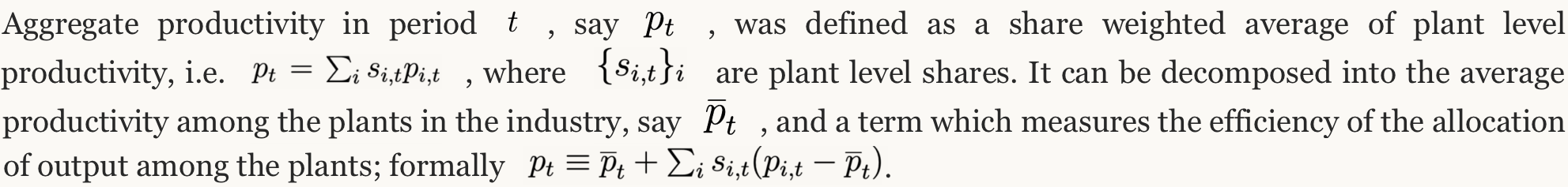
Table 1 presents the results. Partial deregulation started in earnest in 1975 with the reg- istration and certification program. The consent decree was signed in 1982 and the breakup was to be completed by 1984. The table indicates that from 1975 to 1982 there is a reallo- cation of production to more productive plants. In 1983-84 the reorganization caused by the breakup disrupted this process, but post 1984 the allocation rebounds to its prior level and is still increasing at the end of the panel.
The table illustrates two other facts. First notice that prior to deregulation (in 1975) plant level capital was negatively correlated with productivity. Prior to the breakup A.T.& T was the major purchaser of telecommunications equipment. They purchased primarily from their wholly owed subsidiary, Western Electric, which was using dated technology. The breakup induced new entrants (e.g.’s; Ericson, Northern Telecom & Hitachi) and the ”baby bells” turned to them for more modern equipment. Western Electric responded by divesting plants with the older technology.

2. Product Repositioning
Chris Nosko’s thesis (2011) studies the introduction ot the Core 2 Duo chip launched by Intel in 2006. It embodied a major leap in performance and efficiency. The following figures show you how Intel capitalized on its investments.
The first is a snapshot of the price and performance of the chips marketed in June 2006, just prior to the introduction of the Core 2 Duo. The red and blue dots represent AMD’s and Intel’s offerings, respectively. Notice the intense competition for high performance chips with AMD selling the highest priced product at just over $1000 and seven products sold at prices between $1000 and $600.
July sees the introduction of the Core 2 Duo chips indicated with the hollow blue circles. Initially they were offered over a wide range of price/performance points. By October there were no chips sold between $600 to $1000, but there were still two high end older chips, which were removed by January. Nosko shows that Intel’s returns from the Core 2 Duo came from emptying out the middle range of the price/performance products and forcing a choice for either the highest end chip, or a chip with markedly lower performance.
Notice how quickly Intel was able to reposition their chip offerings. Product repositioning is usually ignored in the analysis of the short-run implications of environmental changes (the leading example being merger analysis), but in many industries products can be repositioned very quickly and at little cost. In those industries ignoring product repositioning incentives can lead to extremely faulty predictions even in the very short-run.
A more recent example illustrates this. Wollman (2018) asks what would have happened had GM and Chrysler’s truck divisions not been bailed out during the 2008-2010 recession. He presumes that without the bailout the two truck divisions would have been closed and the analysis asks about the implications of the closures. He notes that trucks are modular; different cabs can be connected to different trailers quickly with very small adjustment costs.
Wollman analyzes the counterfactual closures in different ways. In the first he holds the characteristics of the other truck manufacturers constant and just allows the prices of those trucks to change in response to the closures, as in the standard mode of short run analysis. In the second he allows the other firm’s to first reposition their products in response to the closing, and then chose prices. The implications for welfare of the two analysis are strikingly different; when repositioning is not allowed welfare falls by eleven per cent, but once repositioning is allowed the loss in welfare is under one per cent.
Neither of these studies required a full dynamic analysis of the evolution of the market. They did, however, require two tools not typically needed in static analysis. They needed some way of estimating the cost of repositioning, and because once one allows for repositioning there can be many different outcomes that are Nash equilibria, they required some way of choosing among the possibilities. As illustrated by Pakes et. al.,(2015) moment inequalities generates a simple non-parametric (and therefore reasonably robust) way of estimating the fixed cost. The “multiplicity” problem is mitigated though not solved, by the fact that historical conditions rule out many of the possible equilibria. Both Nosko (2011) and Wollman (2018) use an adaptation of reinforcement learning to choose among the remainder.
3. Transitioning to Dynamics
The empirical work discussed thus far largely relied on using static tools to analyze the implications of different phenomena. These were primarily developments in the analysis of demand systems (see BLP, 1995 and 2004), sometimes in conjunction with production function analysis and/or the tools required to analyze product repositioning. This is often sufficient to track what happened as a result of a prior change in technology (for an excellent recent example see Greico et. al., 2023). However to analyze the implications of environmental change on the development and/or the diffusion of new technologies, and therefore to be able to credibly analyze counterfactuals, we need a dynamic model that incorporates investment and entry possibilities.
The static empirical framework relied on the developments of both, equilibrium notions from theory, and of the econometrics that enabled us to apply these notions in frameworks that incorporated the rich institutional detail needed to generate realistic pictures of markets. We were less successful in adapting the initial dynamic theory models to empirical analysis. I would argue that this is primarily because these models made assumptions which resulted in analytic frameworks that became very complex when faced with the reality of actual market institutions (Formally they combined subgame perfection with assumptions which guaranteed that states evolve as a Markov process. See Maskin and Tirole (1988) for the theory and Ericson and Pakes (1995) for the related applied framework).
The complexity of these models both limited our ability to do dynamic analysis of market outcomes and, perhaps more importantly, led to a question of whether some other model better approximated agents’ behavior. The initial models presumed agents that; ( i) could access a large amount of information, and (ii) either compute or learn an unrealistic number of strategies (some for situations they have never experienced). Allowing for asymmetric information, that is for agents who do not know everything of import to their competitors, mitigates the first problem but just accentuates the complexity of computing policies.
Both theory and empirical work explored a number of ways forward. I want to focus on two of them; (i) use of a weaker notion of equilibrium (one that is less demanding of both decision makers and researchers), and (ii) use of a learning process that mimics how firms respond to change. These are not mutually exclusive. Most learning processes converge to a “rest point” that satisfies Nash conditions and what little empirical work there is, indicates this is also true in data (see Doraszelski et. al. 2018). So one possibility is to use equilibrium conditions to model longer run outcomes and learning models for the transition paths.
The theory models that allowed for weaker notions of equilibrium included Fudenberg and Levine (1993) on self-confirming equilibrium, Osborne and Rubinstein (1998) on procedurally rational players, and Esponda and Pouzo (2016) on Berk-Nash equilibrium (which allows for improper priors). These models were focused on learning about behavior from an unchanging set of payoff relevant state variables. Fershtman and Pakes (2012) introduce the notion of Experienced Based Equilibrium (henceforth EBE) which incorporates similar ideas into a model that allows state variables to evolve with the outcomes of investment and entry processes, as is needed for empirical work. They also provide a learning algorithm which can be used to either compute equilibria or as a model of how firms adapt to new situations.
4. EBE and Empirical Work
Dubois and Pakes (2025), in their study of pharmaceutical advertising in markets for drugs developed to ameliorate four different conditions, provide a way of transitioning from the theoretical EBE framework to empirical work. They first consider an empirical model which only assumes that firms chose advertising to maximize their perceptions of the discounted value of future net cash flows that the advertising dollars will generate. However the empirical model does notrequire that the firms’ perceptions be “correct”, or equilibrium perceptions. That model is used to empirically investigate which variables in the data they the researchers had access to firm’s respond to, and whether the disturbances, which represent the variables that advertising responds to but are not in the available data, are serially correlated. As are most economic variables, the disturbances were highly serially correlated.
The second model assumes that firms decisions condition on the variables uncovered in the empirical model, including state variables that are unobserved by the researcher but evolve as the Markov process estimated in the empirical model. It then computes an EBE that is consistent with these conditioning sets. This allows for asymmetric information (different firms condition on different variables), and assumes that firms” are maximizing given their perceptions and their perceptions of the future are, at least on average, correct. Both the empirical model and the equilibrium model can be fit to the existing data. So we can do an in-sample comparison between them to judge whether the restrictions implicit in the equilibrium model are appropriate.
We distinguish between two types of advertising; direct to consumer advertising (or DTCA) which is predominantly TV advertising, and detailing which involves sending representatives to doctor’s offices. The paper’s goal is to consider what would happen were the rules governing DTCA to change. This requires exploring an out of sample (or counterfactual) environment, including what would happen to detailing if, say, we banned DTCA. Since there is no data from the counterfactual environment, we can not use the empirical model for this. So this is where the more detailed equilibrium model is particularly helpful.
A few of the empirical results are of more general interest to the study of dynamics so I review them here. The first of these concerns the variables that determine the dynamic controls (our advertising variables). The “observable” variable that most effected both types of advertising in all four markets was the derivative of the static profit function with respect to the advertising variable. An optimizing firm with no cognitive or computational constraints would increment its advertising until the expected discounted value of future net cash flows generated by the next unit of advertising just equaled a dollar; i.e. until the derivative of the value function is set equal to one. The firm is not likely to be able to compute that derivative as it requires a correct model of the distribution of possible actions of its competitors in the future and its own responses to that behavior. However the value function is an iterate of the profit function, so the derivative of the profit function is a sensible variable to use to approximate the value function’s derivative.
Notice that I put the word “observable” in quotation marks. The profit variable that we use is constructed from demand and cost estimates. It is not a number found in firm reports. This is crucial, as the demand and cost primitives are combined in the profit function in a way that reflects the closeness of one firm’s product to different competitors and, consequently, to how a change in one aspect of the environment will affect the entire market. As a result the dynamic requires the static tools.
As noted the profit function is determined, in part, by the advertising of all competitors. We found that in addition to the effect of competitors’ advertising through the profit function, the advertising of “close competitors” , had an independent impact on the firms’ advertising (i.e. competitors in the same Anatomical Therapeutic Chemical 4, or ATC4 class). Our markets had between 32 and 57 products over the eight years of data, which were in 3 to 14 ATC4 classes. Also, as expected, advertising falls as patented pharmaceuticals approach the end of their patents lifespan, as the end of exclusivity brings in lower priced generics who may also gain from the advertising.
A final word on in-sample fit. The data contained 38 quarterly periods. Our fits were calculated by conditioning on the first period a drug was advertised and using the advertising models to predict the second period, then using the second period prediction to predict the third period, and continuing in this way for the 38 periods. The serial correlation was strong enough to insure that the initial periods of both models fit extremely well. Perhaps unsurprisingly the empirical model fit better between periods 8 and 20 (though only modestly). More surprisingly the equilibrium model did better thereafter, and increasingly so the farther out the predictions. There are alternative explanations for this. One is that though firms can err in the short run, they do not venture too far off path before correcting themselves. Another is that it is caused by some form of modeling error.
5. Conclusion
Much remains to be done, though I prefer to think of the glass as half full, rather than half empty. We have a better set of models than were available in the past, computers are more powerful, and much more data is available. One word of warning. New issues will arise in trying to model research and other types of investments, and they will require differences in the models used to analyze them.
***
| Citation: Ariel Pakes, Lessons From Empirical Work on Market Dynamics, Network Law Review, Spring 2025. |
References:
- Steve Berry, Jim Levinsohn, and Ariel Pakes (1995) “Automobile Prices in Market Equilibrium,” Econometrica, 63(4): 841-890.
- Steve Berry, Jim Levinsohn, and Ariel Pakes (2004) “Differentiated Products Demand Systems from a Combination of Micro and Macro Data: The New Car Market,” Journal of Political Economy, 112(1): 68-105.
- Uli Doraszelski, Greg Lewis, and Ariel Pakes (2018) “Just Starting Out: Learning and Equilibrium in a New Market,” American Economic Review, 108(3): 565-615.
- Pierre Dubois and Ariel Pakes, 2025; “Pharmaceutical Advertising in Dynamic Equilibrium”,
- Esponda and Pouzo (2016), “Berk-Nash Equilibrium: A Framework for Modeling Agents With Misspecified Models” in Econometrica 84, No. 3, pp. 1093-1130.
- Richard Ericson and Ariel Pakes (1995) “Markov-Perfect Industry Dynamics: A Framework for Empirical Work,” Review of Economic Studies, 62(1): 53-82.
- Chaim Fershtman and Ariel Pakes (2012) “Dynamic Games with Asymmetric Information: A Framework for Empirical Work,” The Quarterly Journal of Economics, 127(4): 1611-1661.
- Paul L.E. Grieco, Charles Murry, Ali Yurukoglu (2023), “The Evolution of Market Power in the U.S. Automobile Industry”, The Quarterly Journal of Economics September 2023 Vol. 139 Issue 2 Pages 1201–1253
- Fundenberg and D. Levine (1993): “Self-Confirming Equilibrium” Econometrica Vol. 61, No. 3, pp. 523-545
- Maskin and J. Tirole (1988): ” A Theory of Dynamic Competition II; Price Competition, Kinked Demand Curves, and Edgeworth Cycles” Econometrica 56(3) pp 571-549.
- Maskin and J. Tirole (1988): “A Theory of Dynamic Oligopoly, I: Overview and Quantity Competition with Large Fixed Costs” Econometrica 56(3) pp 571-599. 549-569.
- Chris Nosko (2011), ” Essays on Technology Markets”, unpublished Ph.D Dissertation Harvard University.
- Steve Olley and Ariel Pakes (1996) “The Dynamics of Productivity in the Telecommunications Equipment Industry,” Econometrica, 64(6): 1263-1297.
- Osborne and A. Rubinstein (1998) “Games with Procedurally Rational Players”, American Economic Review1998, pp834-847.
- Ariel Pakes, Jack Porter, Kate Ho and Joy Ishii (2015) “Moment Inequalities and Their Application,” Econometrica, 83(1): 315-334.
- Thomas Wollman (2018); “Trucks without Bailouts: Equilibrium Product Characteristics for Commercial Vehicles” American Economic Review, 2018, 108(6): 1364-1406